TS Inter 1st Year

Learning these TS Inter 1st Year Maths 1A Formulas Chapter 4 Addition of Vectors will help students to solve mathematical problems quickly.

TS Inter 1st Year Maths 1A Addition of Vectors Formulas

→ Scalar : A physical quantity having magnitude is called a scalar.
E.g. : Length, mass, area, volume, temperature, speed etc.

→ Vector : A physical quantity having both magnitude and direction is called a vector.
Ex : Displacement, velocity, acceleration, force, angular momentum.

→ Modulus of a vector : If a vector \(\overline{\mathrm{AB}}\) is denoted by a̅ then |a̅|. denote the length oi the vector of a̅ also |a̅| is called the magnitude or modulus of a vector a .

→ Collinear or parallel vectors : Vectors along the same line or along the parallel line are called collinear vectors. In figure \(\overline{\mathrm{AB}}, \overline{\mathrm{BC}}, \overline{\mathrm{CA}}\) are collinear vectors. Two vectors a̅ b̅ are parallel or collinear iff a̅ = tb̅ . t ∈ R.

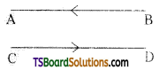
→ Like vectors: Collinear or parallel vectors having the same direction are called like vectors.

→ Unlike vectors:
Collinear or parallel vectors having opposite direction are called unlike vectors.

→ Unit vector:
A vector whose modulus is unity is called a unit vector. The unit vector in the direction of vector a̅ is denoted by a̅̂. Thus modulus of |a̅̂| = 1.

• Unit vector in the direction of a̅ is \(\frac{\overline{\mathrm{a}}}{|\overline{\mathrm{a}}|}\).
• Unit vector in the opposite direction of a̅ is \(\frac{-a}{|\bar{a}|}\).

→ Position vector : If a point ‘O’ is fixed as origin in the plane and ‘A’ is any point then \(\overline{\mathrm{OA}}\) is called the position vector of A’ with respect to ‘O’.

→ Triangle law of addition of vectors: In a triangle OAB, let \(\overline{\mathrm{OA}}\) = a̅, \(\overline{\mathrm{AB}}\) = b̅ then the resultant vector \(\overline{\mathrm{OB}}\) is defined as \(\overline{\mathrm{OB}}=\overline{\mathrm{OA}}+\overline{\mathrm{AB}}\) = a̅ + b̅.
This is known as triangle law of addition of vectors.

→ Section formula:

• Let A and B be two points with position vectors a̅ and b̅ respectively. Let ‘C’ be a point dividing AB internally in the ratio m : n. The position of ‘C’ is \(\overline{O C}=\frac{m b+n a}{m+n}\)
• Let A and B be two points with position vectors a̅ and b̅. Let be a point dividing the line segment AB externally in the ratio in : n then the position vector of C is given by \(\overline{\mathrm{OC}}=\frac{\mathrm{mb}-n \bar{a}}{m-n}\)

→ The position vector of the midpoint of the line segment joining two vectors with position vector is \(\frac{\bar{a}+\bar{b}}{2}\).

→ Coplanar vectors: Two or more vectors are said to be coplanar if they lie on the same plane.

• The vectors a̅, b̅, c̅ are said to be coplanar iff [a̅ b̅ c̅] = 0.
• Four points A, B. C. D are said to be coplanar iff \(\left[\begin{array}{lll}
  \overline{\mathrm{AB}} & \overline{\mathrm{AC}} & \overline{\mathrm{AD}}
  \end{array}\right]\) = 0.
• Three vectors a̅, b̅, c̅ are said to be linearly dependent iff [a̅ b̅ c̅] = 0.
• Three vectors a̅, b, c̅ are said to be linearly independent iff [a̅ b̅ c̅] = 0.

→ Vector equations of a straight line :

• The vector equation of the straight line passing through the point A (a̅) and parallel to the vector b̅ is r̅ = a̅ + tb̅ , t ∈ R.
• The vector of the line passing through origin ‘O’ and parallel to the vector b̅ is r̅ = tb̅, t ∈ R.
  Cartesian form : Cartesian equation for the line equation passing through A (x₁, y₁, z₁) and parallel to the vector b̅ = li + mj + nk is \(\frac{x-x_1}{l}=\frac{y-y_1}{m}=\frac{z-z_1}{n}\)
• The vector equat ion of the line passing through the points A (a) and B(b) is r = (1 – t) a̅ + tb̅. t ∈ R.
  Cartesian form : Cartesian equation for the line through A(x₁, y₁, z₁) and B(x₂, y₂, z₂) is \(\frac{\mathrm{x}-\mathrm{x}_1}{\mathrm{x}_2-\mathrm{x}_1}=\frac{\mathrm{y}-\mathrm{y}_1}{\mathrm{y}_2-\mathrm{y}_1}=\frac{\mathrm{z}-\mathrm{z}_1}{\mathrm{z}_2-\mathrm{z}_1}\)

→ Vector equations of a plane :

• The vector equation of the plane passing through the points A(a̅) and parallel to the vectors b̅ & c̅ is r̅ = a̅ + tb̅ + sc̅ : t. s ∈ R.
• The equation of the plane passing through the points A(a̅).B(b̅) and parallel to the vector c is r̅ = (1 – t) a̅ + tb + sc̅ ; t, s ∈ R.
• The equation of the plane passing through three non-collinear points A(a̅), B(b̅) and C(c̅) is r̅ = (1 – t – s)a̅ + tb̅ + sc̅ ; t, s ∈ R.

→ Linear combinations : Let \(\overline{a_1}, \overline{a_2}, \ldots \ldots, \overline{a_n}\) be n vectors and l₁, l₂, …………. l_n be n scalars.
Then \(l_1 \overline{\mathrm{a}_1}+l_2 \overline{\mathrm{a}_2}, \ldots \ldots \ldots+l_{\mathrm{n}} \overline{\mathrm{a}_{\mathrm{n}}}\) is called a linear combination of \(\overline{\mathrm{a}_1}, \overline{\mathrm{a}_2}, \ldots \overline{\mathrm{a}_{\mathrm{n}}}\).

Learning these TS Inter 1st Year Maths 1A Formulas Chapter 6 Trigonometric Ratios up to Transformations will help students to solve mathematical problems quickly.

TS Inter 1st Year Maths 1A Trigonometric Ratios up to Transformations Formulas

→ sin θ, cos θ, tan θ, cot θ, cosec θ and sec θ are called trigonometric functions. The reciprocals of sin θ, cos θ, tan θ are cosec θ, sec θ and cot θ respectively.

→ The main identities are sin²θ + cos²θ =1, sec²θ – tan²θ = 1 and cosec²θ – cot²θ = 1.

→ The bounds for sin θ, cos θ and sec θ are |sin θ| ≤ 1, |cosec θ| ≤ 1 and |sec θ| ≥ 1.

→ The three main tables are given by
Table 1 :

→ Using “All Silver Tea Cups”, the following tables may be comitted to memory.
Table 2:

Table 3:

→ sin 0° = 0 = cos 90°

• sin 15° = \(\left(\frac{\sqrt{3}-1}{2 \sqrt{2}}\right)\) = cos 75°, sin 18° = \(\left(\frac{\sqrt{5}-1}{4}\right)\) = cos 72°
• sin 36° = \(\left(\frac{\sqrt{10}-2 \sqrt{5}}{4}\right)\) = cos 54°, sin 54° = \(\left(\frac{\sqrt{5}+1}{4}\right)\) = cos 36°
• sin 72° = \(\left(\frac{\sqrt{10+2 \sqrt{5}}}{4}\right)\) = cos 18°
• sin 75° = \(\left(\frac{\sqrt{3}+1}{2 \sqrt{2}}\right)\) = cos 15°
• tan 15° = 2 – √3 , tan 75° = 2 + √3

→ Any non constant function f: R → R is said to be Periodic” if there exists a real number p (* 0) such that f (x + p) = f(x) for each x e R. The least positive value of p with this period is called the “Period of f”.

→ (a) If f (x) is a periodic function with period p then f(ax +b) is also a periodic function with period \(\left(\frac{p}{|a|}\right)\)
(b) If y = f(x), y = g(x) are periodic functions with l, m as the periods respectively then h(x) = a f(x) + b g(x) where a, b R is a periodic function and LCM of {l, m} if exist is a period of h.
(c) The period of sin x, cosec x, cos x and sec x is 2π.
(d) The period of tan x and cot x is π.

→ (a) Range of a sin x + b cos x is \(\left[-\sqrt{a^2+b^2}, \sqrt{a^2+b^2}\right]\)
(b) Range of a sin x + b cos x + c is \(\left[c-\sqrt{a^2+b^2}, c+\sqrt{a^2+b^2}\right]\)

→ (a) sin(A ± B) = sin A cos B ± cos A sin B
(b) cos(A ± B) = cos A cos B ∓ sin A sin B
(c) tan (A ± B) = \(\frac{\tan A \pm \tan B}{1 \mp \tan A \tan B}\)
(d) cot (A ± B) = \(\frac{\cot A \cot B \pm 1}{\cot B \mp \cot A}\)
(e) sin (A + B) sin (A – B) = sin²A – sin²B = cos²B – cos²A
(f) cos (A + B) cos (A – B) = cos2A – sin’B = cos2B – sin2A

→ (a) sin (A + B + C) = sin A cos B cos C + cos A sin B cos C + cos A cos B sin C – sin A sin B sin C
(b) cos (A + B + C) = cos A cos B cos C + cos A sin B sin C – sin A cos B sin C – sin A sin B cos C
(c) tan (A + B + C) = \(\frac{\sum \tan A-\pi \tan A}{1-\sum \tan A \tan B}\)

→ (a) sin 2A = 2 sinA cos A, sinA = 2 sin\(\frac{\mathrm{A}}{2}\) cos \(\frac{\mathrm{A}}{2}\)
(b) cos 2A = cos²A – sin²A = 1 – 2 sin²A = 2 cos²A – 1
cos A = cos² \(\frac{\mathrm{A}}{2}\) – sin² \(\frac{\mathrm{A}}{2}\) = 1 – 2 sin²\(\frac{\mathrm{A}}{2}\) = 2 cos² \(\frac{\mathrm{A}}{2}\) – 1
(c) tan 2A = \(\frac{2 \tan A}{1-\tan ^2 A}\), tan A = \(\frac{2 \tan \frac{A}{2}}{1-\tan ^2 \frac{A}{2}}\) (\(\frac{A}{2}\), A are not odd multiples of \(\frac{\pi}{2}\))
(d) cot 2A = \(\frac{\cot ^2 A-1}{2 \cot A}\), cot A = \(\frac{\cot ^2 \frac{A}{2}-1}{2 \cot \frac{A}{2}}\) (A is not an integral multiple of π)
(e) sin 2A = \(\frac{2 \tan A}{1+\tan ^2 A}\), sin A = \(\frac{2 \tan \frac{A}{2}-1}{1+\tan ^2 \frac{A}{2}}\) (\(\frac{A}{2}\) is not an integral multiple of \(\frac{\pi}{2}\))
(f) cos 2A = \(\frac{1-\tan ^2 \mathrm{~A}}{1+\tan ^2 \mathrm{~A}}\), cos A = \(\frac{1-\tan ^2 \frac{A}{2}}{1+\tan ^2 \frac{A}{2}}\)

→ (a) sin 3A = 3 sin A – 4 sin³A
(b) cos 3A = 4cos³A – 3 cos A
(c) tan 3A = \(\frac{3 \tan A-\tan ^3 A}{1-3 \tan ^2 A}\)
(d) cot 3A = \(\frac{3 \cot A-\cot ^3 A}{1-3 \cot ^2 A}\)

→ Sums into formulae:
(a) sin (A + B) + sin (A – B) = 2 sin A cos B
(b) sin(A + B) – sin (A – B) = 2 cos A sin B
(c) cos (A + B) – cos (A – B) = 2 cos A cos B
(d) cos (A – B) – cos (A + B) = 2 sin A sin B

→ (a) sin C + sin D = 2 sin \(\left(\frac{C+D}{2}\right)\) cos \(\left(\frac{C-D}{2}\right)\)
(b) sin C – sin D = 2 cos\(\left(\frac{C+D}{2}\right)\) sin \(\left(\frac{C-D}{2}\right)\)
(c) cos C + cos D = 2 cos\(\left(\frac{C+D}{2}\right)\) cos \(\left(\frac{C-D}{2}\right)\)
(d) cos C – cos D = 2 sin \(\left(\frac{C+D}{2}\right)\) sin \(\left(\frac{D-C}{2}\right)\)

→ (a) sin A = ±\(\sqrt{\frac{1-\cos 2 A}{2}}\)
(b) cos A = ±\(\sqrt{\frac{1+\cos 2 A}{2}}\)
(c) tan A = ±\(\pm \sqrt{\frac{1-\cos 2 A}{1+\cos 2 A}}\), if A is not an odd multiple of \(\frac{\pi}{2}\)

→ (a) sin \(\frac{A}{2}=\pm \sqrt{\frac{1-\cos A}{2}}\)
(b) cos \(\frac{A}{2}=\pm \sqrt{\frac{1+\cos A}{2}}\)
(c) tan\(\frac{A}{2}=\pm \sqrt{\frac{1-\cos A}{1+\cos A}}\), if A is not an odd mutiple of π.

→ (a) sin x and cos x are continuous functions on IR.
(b) tan x is discontinuous at x = (2n – 1) \(\frac{\pi}{2}\), n ∈ Z
(c) sec x is discontinuous at x = (2x + 1) \(\frac{\pi}{2}\), n ∈ Z
(d) cosec x is discontinuous at x = nπ, n ∈ Z

Learning these TS Inter 1st Year Maths 1A Formulas Chapter 7 Trigonometric Equations will help students to solve mathematical problems quickly.

TS Inter 1st Year Maths 1A Trigonometric Equations Formulas

→ Trigonometric equation :
An equation involving trigonometric functions is called a trigonometric equation.
Ex – 1 : a cos² θ – b sin θ + c = 0
Ex – 2 : a cos θ + b sin θ + c = 0
Ex – 3 : a tan θ + b sec θ + c = 0

→ General solution (or) solution set:
The set of all values of θ which satisfy a trigonometric equation f(θ) = 0 is called general solution (or) solution set of f(θ) = 0.

→ Principle value:
1. There exists a unique value of θ in \(\left[\frac{-\pi}{2}, \frac{\pi}{2}\right]\) satisfying sin θ = k, k ∈ R. |k| ≤ 1. This value of θ is called principle value of θ (or) principle solution of sin θ = k.
Ex :

• Principle solution of sin θ = \(\frac{1}{2}\) is \(\frac{\pi}{6}\).
• Principle solution of sin θ = \(\frac{-1}{\sqrt{2}}\) is \(\frac{-\pi}{4}\).

2. There exists a unique value of θ in [0, n] satisfying cos θ = k. k ∈ R. |k| < 1. This value of θ is called principle value of θ (or) principle solution of cos θ = k.
Ex :

• Principle solution of cos θ = \(\frac{1}{\sqrt{2}}\) is \(\frac{\pi}{4}\).
• Principle solution of cos θ = \(\frac{-1}{2}\) is \(\frac{2 \pi}{3}\).

3. There exists a unique value of θ in \(\left(\frac{-\pi}{2}, \frac{\pi}{2}\right)\) satisfying tan θ = k, k ∈ R. This value of θ is called principle value of θ (or) principle solution of tan θ = k.
Ex :

• Principle solution of tan θ = √3 is \(\frac{\pi}{3}\).
• Principle solution of tan θ = \(\frac{-1}{\sqrt{3}}\) is \(\frac{-\pi}{6}\)

→ General solutions of trigonometric equations:

Learning these TS Inter 1st Year Maths 1A Formulas Chapter 8 Inverse Trigonometric Functions will help students to solve mathematical problems quickly.

TS Inter 1st Year Maths 1A Inverse Trigonometric Functions Formulas

→ sin^-1(sin θ) = θ, if θ ∈ \(\left[\frac{-\pi}{2}, \frac{\pi}{2}\right]\)

→ sin (sin^-1x) = x, if x ∈ [-1, 1]

→ cos^-1(cos θ) = θ, if θ ∈ [0, π]

→ cos (cos^-1x) = x, if x ∈ [-1, 1]

→ tan^-1(tan θ) = θ, if θ ∈ \(\left[\frac{-\pi}{2}, \frac{\pi}{2}\right]\)

→ tan(tan^-1x) = x, if x ∈ R

→ cot^-1(cot θ) = θ, if θ ∈ (0, π)

→ cot(cot^-1x) = x, if x ∈ R

→ sin^-1 (- x) = – sin^-1 x if x ∈ [-1, 1]

→ cos^-1(- x) = π – cos^-1 x if x ∈ [-1, 1]

→ tan^-1 (- x) = – tan^-1 x, if x ∈ R

→ cot^-1 (- x) = π – cot^-1 x if x ∈ R

→ sin^-1 x – cos 1 x = \(\frac{\pi}{2}\) , if x ∈ [-1, 1]

→ tan^-1x + cot^-1x = \(\frac{\pi}{2}\), for any x ∈ R

→ sec^-1x + cosec^-1x = \(\frac{\pi}{2}\) , if x ∈ (-∞, -1] ∪ [1, ∞)

→ sin^-1x = cosec^-1\(\left(\frac{1}{x}\right)\) for x ∈ [-1, 0) ∪[1, ∞)

→ cos^-1x = sec^-1\(\left(\frac{1}{x}\right)\) for x ∈ [-1, 0) ∪(0, 1]

→ cot^-1x = tan^-1\(\frac{1}{x}\) if x > 0

→ cot^-1x = + tan^-1\(\frac{1}{x}\) , if x < 0

→ sin^-1x + sin^-1y = sin^-1 (x\(\sqrt{1-y^2}\) + y\(\sqrt{1-x^2}\)) if x, y ∈ [0, 1] and x² + y² < 1

→ sin^-1x + sin^-1 y = π – sin^-1 (x\(\sqrt{1-y^2}\) + y\(\sqrt{1-x^2}\)) if x, y ∈ [0, 1] and x² + y² > 1

→ sin^-1x – sin^-1y = sin^-1(x\(\sqrt{1-y^2}\) – y\(\sqrt{1-x^2}\)) if x. y ∈ [0, 1]

→ cos^-1x + cos^-1y = cos^-1(xy – \(\sqrt{1-x^2} \sqrt{1-y^2}\)) if x, y ∈ [0, 1 ]

→ cos^-1x – cos^-1y = cos^-1(xy + \(\sqrt{1-x^2} \sqrt{1-y^2}\)) if 0 ≤ x ≤ y ≤ 1

→ tan^-1x – tan^-1y = tan^-1\(\left(\frac{x-y}{1+x y}\right)\) if x > 0, y >0 (or) x < 0, y < 0

→ 2sin^-1x = sin^-1 (2x\(\sqrt{1-\mathrm{x}^2}\))

→ 2cos^-1x = cos^-1(2x² – 1)

→ 2tan^-1x = tan^-1\(\left(\frac{2 x}{1-x^2}\right)\)

→ 3sin^-1x = sin^-1(3x -4x³)

→ 3cos^-1x = cos^-1(4x³ – 3x)

→ 3tan^-1x = tan^-1\(\left(\frac{3 x-x^3}{1-3 x^2}\right)\)

Learning these TS Inter 1st Year Maths 1A Formulas Chapter 9 Hyperbolic Functions will help students to solve mathematical problems quickly.

TS Inter 1st Year Maths 1A Hyperbolic Functions Formulas

→ Hyperbolic Functions:

→ Inverse Hyperbolic Functions:

→ Hyperbolic Identities:

• cosh²x – slnh²x = 1
• sech²x – tanh²x = 1
• coth²x – cosech²x = 1
• sinh(2x) = 2sinhx coshx
• cosh(2x) = cosh²x + sinh²x = 1 + 2sinh²x = 2cosh²x – 1

→ sinh (- x) = – sin hx

→ cosh (- x) = cosh x

→ tanh(-x)= -tanhx

→ coth(-x) = -coth x

→ cosech(-x) = -cosech x

→ sech(-x) = sech x

→ sinh (x + y) = shih x . cosh y + cosh x sin h y

→ cosh (x + y) = cosh x. cosh y + sin h x sinb y

→ sinh(x – y) sinhx.cosh y – cosh x sinh y

→ cosh(x – y)=coshx.coshy – sinhxsinhy

→ tanh (x + y) = \(\frac{\tanh x+\tanh y}{1+\tanh x \tanh y}\)

→ tanh (x – y) = \(\frac{\tanh x-\tanh y}{1-\tanh x \tanh y}\)

→ sinh3x = 3sinhx + 4sinh³x

→ cosh3x = 4cosh³x – 3coshx

→ tanh3x = \(\frac{3 \tanh x+\tanh ^3 x}{1+3 \tanh ^2 x}\)

Learning these TS Inter 1st Year Maths 1A Formulas Chapter 10 Properties of Triangles will help students to solve mathematical problems quickly.

TS Inter 1st Year Maths 1A Properties of Triangles Formulas

→ In any ΔABC, \(\frac{a}{\sin A}=\frac{b}{\sin B}=\frac{c}{\sin C}\) = 2R where a, b, c are the lengths of sides BC, CA and AB of a triangle ABC. A, B, C are the angles at the vertices of ΔABC, and R is the circum radius of the ΔABC. This is called the SINE RULE.

→ In any ΔABC,

• a² = b² + c² – 2bc cos A
• b² = c² + a² – 2ca cos B
• c² = a² + b² – 2ab cos C is the COSINE RULE.

→ The angles A, B, C can be found by the formulae

• cos A = \(\frac{b^2+c^2-a^2}{2 b c}\)
• cos B = \(\frac{c^2+a^2-b^2}{2 c a}\)
• cos C = \(\frac{a^2+b^2-c^2}{2 a b}\)

→ In any ΔABC,

• a = b cos C + c cos C
• b = a cos C + c cos A
• c = a cos B + b cos A (projection formulae)

→ tan\(\left(\frac{B-C}{2}\right)=\frac{b-c}{b+c}\) cot\(\frac{A}{2}\) (or) tan\(\left(\frac{c-A}{2}\right)=\frac{c-a}{c+a}\)cot\(\frac{B}{2}\) (or)
tan\(\left(\frac{A-B}{2}\right)=\frac{a-b}{a+b}\) cot \(\frac{C}{2}\) is the Napier’s analogy

→ If a + b + c = 2s which is the perimeter of ΔABC then
sin\(\frac{A}{2}=\sqrt{\frac{(s-b)(s-c)}{b c}}\), sin\(\frac{B}{2}=\sqrt{\frac{(s-a)(s-c)}{a c}}\) and sin\(\frac{c}{2}=\sqrt{\frac{(s-a)(s-b)}{a b}}\)
cos\(\frac{A}{2}=\sqrt{\frac{s(s-a)}{b c}}\), cos\(\frac{\mathrm{B}}{2}=\sqrt{\frac{s(s-b)}{a c}}\), cos \(\frac{c}{2}=\sqrt{\frac{s(s-c)}{a b}}\) and
tan\(\frac{A}{2}=\sqrt{\frac{(s-b)(s-c)}{s(s-a)}}\), tan\(\frac{B}{2}=\sqrt{\frac{(s-a)(s-c)}{s(s-b)}}\), tan\(\frac{c}{2}=\sqrt{\frac{(s-a)(s-b)}{s(s-c)}}\)

→ Area of ΔABC Δ = \(\frac{1}{2}\)bc sin A = \(\frac{1}{2}\)ca sin B = \(\frac{1}{2}\)ab sin C
= \(\sqrt{s(s-a)(s-b)(s-c)}=\frac{a b c}{4 R}\) = 2R sin A sin B sin C

→ If ‘r’ is the radius of incircle of ΔABC; r₁, r₂, r₃ are the radii of excircle then
r = \(\frac{\Delta}{s}\), r₁ = \(\frac{\Delta}{s-a}\), r₂ = \(\frac{\Delta}{s-b}\) and r₃ = \(\frac{\Delta}{s-c}\)

→ Also r = 4R sin\(\frac{A}{2}\)sin\(\frac{B}{2}\)sin\(\frac{C}{2}\)

• r₁ = 4R sin\(\frac{A}{2}\)cos\(\frac{B}{2}\)cos\(\frac{C}{2}\)
• r₂ = 4R sin\(\frac{B}{2}\) cos\(\frac{C}{2}\) cos\(\frac{A}{2}\)
• r₃ = 4R sin\(\frac{C}{2}\) cos\(\frac{A}{2}\) cos\(\frac{B}{2}\)

→ In any ΔABC, \(\frac{a+b}{c}=\frac{\cos \left(\frac{A-B}{2}\right)}{\sin \frac{C}{2}}\)
\(\frac{b+c}{a}=\frac{\cos \left(\frac{B-C}{2}\right)}{\sin \frac{A}{2}}\)
and \(\frac{c+a}{b}=\frac{\cos \left(\frac{C-A}{2}\right)}{\sin \frac{B}{2}}\)

Learning these TS Inter 1st Year Maths 1A Formulas Chapter 3 Matrices will help students to solve mathematical problems quickly.

TS Inter 1st Year Maths 1A Matrices Formulas

→ Matrix: If the real or complex numbers are arranged in the form of a rectangular or square array consisting the complex numbers in horizontal and vertical lines, then that arrangement is called a matrix.
Ex: A = \(\left[\begin{array}{ccc}
1 & 2 & 4 \\
3 & 0 & -6
\end{array}\right]\), B = \(\left[\begin{array}{cc}
1 & 2 \\
4 & -3
\end{array}\right]\)

→ Order of a matrix: A matrix ‘A1 is said to be of type (or) order (or) size m × n (read as m by n), if the matrix A’ has m rows and n’ columns.

→ Square matrix: A matrix ‘A’ is said to be a square matrix if the number of rows in A is equal to the number of columns in A.
Ex: \(\left[\begin{array}{cc}
1 & -1 \\
0 & 4
\end{array}\right]\)_2×2
\(\left[\begin{array}{ccc}
2 & 0 & 1 \\
4 & -1 & 2 \\
7 & 6 & 9
\end{array}\right]\)_2×2

→ Trace of a matrix : If ‘A’ is a square matrix then the sum of elements in the principle diagonal of A’ is called trace of A’. It is denoted by tra A .
Ex: A = \(\left[\begin{array}{ccc}
2 & 0 & 1 \\
4 & -1 & 2 \\
7 & 6 & 9
\end{array}\right]\)
The elements of the principle diagonal = 2, – 1, 9
Tra (A) = 2 + (- 1) + 9 = 10.

→ Null matrix : A matrix ‘A’ is said to be a zero matrix or null matrix of every element of A is equal to zero.
Ex: O₂ = \(\left[\begin{array}{ll}
0 & 0 \\
0 & 0
\end{array}\right]\)
O_3×2 = \(\left[\begin{array}{ll}
0 & 0 \\
0 & 0 \\
0 & 0
\end{array}\right]\)

→ Upper triangular matrix: A square matrix A = [a_ij]_n×n is said to be an upper triangular matrix if a_ij, = 0, whenever i > i.
Ex: \(\left[\begin{array}{ccc}
2 & -1 & 5 \\
0 & 3 & 6 \\
0 & 0 & 1
\end{array}\right]_{3 \times 3}\)

→ Lower triangular matrix :
A square matrix A = [a_ij]_n×n is said to he a lower triangular matrix if a_ij, = 0 whenever i < j .
Ex: \(\left[\begin{array}{ccc}
2 & 0 & 0 \\
1 & 3 & 0 \\
5 & 4 & 6
\end{array}\right]_{3 \times 3}\)

→ Triangular matrix : A square matrix. A is said to be a triangular matrix ifA is either an upper triangular matrix or a lower triangular matrix.
Ex: \(\left[\begin{array}{ccc}
-1 & 0 & 0 \\
0 & 3 & 0 \\
7 & 5 & 2
\end{array}\right]_{3 \times 3}\)

→ Diagonal matrIx : A square matrix, A is said to be a diagonal matrix if A is both upper triangnlar and lower triangular matrix. (or) A square matrix in which every element is equal to zero except those of principle diagonal of the matrix Is a diagonal matrix.
Ex: \(\left[\begin{array}{ccc}
2 & 0 & 0 \\
0 & 3 & 0 \\
0 & 0 & -1
\end{array}\right]_{3 \times 3}\)

→ Scalar matrix : A diagonal matrix, A is said to be a scalar matrix if all elements in the principle diagonal are equal.
Ex: \(\left[\begin{array}{ll}
2 & 0 \\
0 & 2
\end{array}\right]_{2 \times 2}\)
\(\left[\begin{array}{lll}
3 & 0 & 0 \\
0 & 3 & 0 \\
0 & 0 & 3
\end{array}\right]_{3 \times 3}\)

→ Unit matrix : A diagonal matrix is said to be a unit matrix if every element in the principle diagonal is equal to unity. It is denoted by 1.
Ex: I₂ = \(\left[\begin{array}{ll}
1 & 0 \\
0 & 1
\end{array}\right]\)
I₃ = \(\left[\begin{array}{lll}
1 & 0 & 0 \\
0 & 1 & 0 \\
0 & 0 & 1
\end{array}\right]\)

→ Transpose of a matrix: The matrix obtained by changing the rows of a given matrix, A into columns is called transpose of ‘A’. It is denoted by A^T or A’.
Ex: A = \(\left[\begin{array}{ccc}
2 & 3 & -1 \\
1 & 2 & 3
\end{array}\right]\) then A^T = \(\left[\begin{array}{cc}
2 & 1 \\
3 & 2 \\
-1 & 3
\end{array}\right]\)

→ Symmetric matrix : A square matrix, A is said to be a symmetric matrix, if A^T = A.
Ex: If A = \(\left[\begin{array}{lll}
2 & 3 & 1 \\
3 & 4 & 5 \\
1 & 5 & 7
\end{array}\right]\), then A^T = \(\left[\begin{array}{lll}
2 & 3 & 1 \\
3 & 4 & 5 \\
1 & 5 & 7
\end{array}\right]^{\mathrm{T}}=\left[\begin{array}{lll}
2 & 3 & 1 \\
3 & 4 & 5 \\
1 & 5 & 7
\end{array}\right]\) = A
A is a symmetric matrix.

→ Skew symmetric matrix : A square matrix A’ is said to be a skew symmetric matrix, if A^T = – A.
Ex: A = \(\left[\begin{array}{ccc}
0 & 1 & -2 \\
-1 & 0 & 3 \\
2 & -3 & 0
\end{array}\right]\), then AT = \(\left[\begin{array}{ccc}
0 & 1 & -2 \\
-1 & 0 & 3 \\
2 & -3 & 0
\end{array}\right]^{\mathrm{T}}=\left[\begin{array}{ccc}
0 & -1 & 2 \\
1 & 0 & -3 \\
-2 & 3 & 0
\end{array}\right]=\left[\begin{array}{ccc}
0 & 1 & -2 \\
-1 & 0 & 3 \\
2 & -3 & 0
\end{array}\right]\) = -A
A is a skew symmetric matrix.

→ Adjoint of a matrix : The transpose of the matrix obtained by replacing the elements of a square matrix. A by the corresponding cofactors is called the adjoint matrix of A. It is denoted by Adi A or adj A.

→ Inverse of a square matrix : A sqiictre matrix A is said to be an invertible matrix, if there exists a square matrix, B such that AB = BA = I. The matrix B is called inverse of A’.
If A is a non-singular matrix, then A is invertible and A^-1 = \(\frac{{adj} A}{{det} A}\)

→ Sub matrix : A matrix obtained by deleting some rows or columns or both of a matrix is called a sub matrix of the given matrix.
Ex: If A = \(\left[\begin{array}{cc}
1 & 2 \\
-1 & 2
\end{array}\right] \cdot\left[\begin{array}{lll}
1 & 2 & 3 \\
2 & 3 & 1
\end{array}\right] \cdot\left[\begin{array}{ll}
2 & 3 \\
3 & 1 \\
2 & 0
\end{array}\right]\) then some matrices of A are \(\left[\begin{array}{cc}
1 & 2 \\
-1 & 2
\end{array}\right] \cdot\left[\begin{array}{lll}
1 & 2 & 3 \\
2 & 3 & 1
\end{array}\right] \cdot\left[\begin{array}{ll}
2 & 3 \\
3 & 1 \\
2 & 0
\end{array}\right]\), [0]

→ Rank of a matrix : Let ‘A’ be a non zero matrix. The rank of A is defined as the maximum of the orders of the non singular square sub-matrices of A. The rank of a null matrix is defined ^ as zero. The rank of a matrix A is denoted by rank [A].

→ Rank of 3 × 3 matrix : Suppose A is a non-zero 3 × 3 matrix, then

• If A is a non – singular then its rank is 3.
• If A is a singular matrix and if at least one of its 2 × 2 sub matrix is non-singular, then the rank of A is 2.
• If A is a singular matrix and every 2×2, sub matrix is also singular, then the rank of ’A’ is 1.

→ Properties of matrices :

• If A and B are two matrices of same type, then A + B = B + A.
• If A, B and C are three matrices of same type then (A + B) + C = A + (B + C).
• If confirmability is assured for the matrices A, B and C then A(BC) = (AB)C.
• If confirmability is assured for the matrices A, B and C then
  (a) A(B + C) = AB + AC
  (b) (B + C) A = BA + CA.
• If A is any matrix then (A^T)^T = A.
• If A and B are two matrices of same type then (A + B)^T = A^T + B^T.
• If A and B are two matrices for which confirmability for multiplication is assured then (AB)^T = B^T. A^T.
• If I is the identity matrix of order n then for every square matrix A of order n. AI = IA = A.
• If A is an invertible matrix then A^-1 is also invertible and (A^-1)^-1 = A.
• If A and B are two invertible matrices of same type then AB is also invertible and (AB)^-1 = B^-1. A^-1.
• If A is an invertible matrix then A is also invertible and (A^T)^-1 = (A^-1)^T

→ Methods of solving linear equations :
1. Cramer’s rule : Let a₁x + b₁y + c₁z = d₁
a₂x + b₂y + c₂z = d₂
a₃x + b₃y + c₃z = d₃
be a system of linear equations

2. Matrix inversion method : If ‘A’ is a non-singular matrix then the solution of AX’ = B is X = A^-1 B.

3. Gauss Jordan method : Let a₁x + b₁y + c₁z = d₁
a₂x + b₂y + c₂z = d₂
a₃x + b₃y + c₃z = d₃
be a system of linear equations. If the augmented matrix \(\left[\begin{array}{llll}
\mathrm{a}_1 & \mathrm{~b}_1 & \mathrm{c}_1 & \mathrm{~d}_1 \\
\mathrm{a}_2 & \mathrm{~b}_2 & \mathrm{c}_2 & \mathrm{~d}_2 \\
\mathrm{a}_3 & \mathrm{~b}_3 & \mathrm{c}_3 & \mathrm{~d}_3
\end{array}\right]\) can be reduced to the form \(\left[\begin{array}{llll}
1 & 0 & 0 & \alpha \\
0 & 1 & 0 & \beta \\
0 & 0 & 1 & \gamma
\end{array}\right]\) by using elementary row transformations then x = α, y = β, z = γ, i.e., unique solution is the solution.

i) In the above matrix \(\left[\begin{array}{llll}
1 & 0 & 0 & \alpha \\
0 & 1 & 0 & \beta \\
0 & 0 & 1 & \gamma
\end{array}\right]\) is called final matrix of the system of equations.

ii) In the final matrix, if ‘O’ is obtained in place of 1 and in the same rows last element α or β or γ is
a) ‘O’ then the system has infinite number of solutions.
b) non-zero then the system of equations has no solution.

→ The system of non-homogeneous equations AX = D has

• a unique solution if rank [A] = rank [AD] = 3
• Infinitely many solutions if rank [A] = rank [AD] < 3
• No solution if rank [A] * rank [AD],

→ The system of homogeneous equations AX = O has

• The trivial solution only if Rank [A] = 3 = The number of unknowns (variables)
• An infinite number of solutions (non-trivial solution), if Rank of A less than the number of unknowns (variables) < 3.

Learning these TS Inter 1st Year Maths 1A Formulas Chapter 2 Mathematical Induction will help students to solve mathematical problems quickly.

TS Inter 1st Year Maths 1A Mathematical Induction Formulas

→ Principle of finite Mathematical Induction : Let S(n) be a statement of a result for each n ∈ N. If

• S(1) is true
• S(K) is true ⇒ S(K + 1) is also true then S(n) is true ∀ n ∈ N. (Set of natural numbers = N).

→ Principle of complete Mathematical Induction : Let S(n) be a statement for each n ∈ N. If

• S(T) is true
• S(1), S(2), S(3), ……….. S(K) are true ⇒ S(K + 1) is true, then S(n) is true, ∀ n ∈ N.

→ Useful formulae:

• 1 + 2 + 3 + ………. + n = \(\frac{n(n+1)}{2}\)
• 1² + 2² + 3² + ……….. + n² = \(\frac{n(n+1)(2 n+1)}{6}\)
• 1³ + 2³ + 3³ + ………… + n³ = \(\frac{n^2(n+1)^2}{4}\)
• The nth term of the arithmetic progression (A.P.) is t_n = a + (n – 1) d
• The sum f n terms of the arithmetic progression (A.P.) is S_n = \(\frac{n}{2}\) [2a + (n – 1) d]
• The nth term of the geometric progression (G.P.) is t_n = a. r^n-1
• The sum of the n terms in G.P is S_n = \(\frac{a\left(r^n-1\right)}{r-1}\). r > 1
• Sum of the first n’ odd natural numbers : 1 + 3 + 5 + ……………….. + (2n – 1) = n²
• Sum of the first n’ even natural numbers : 2 + 4 + 6 + …………….. + (2n) = n (n + 1)

Learning these TS Inter 1st Year Maths 1A Formulas Chapter 1 Functions will help students to solve mathematical problems quickly.

TS Inter 1st Year Maths 1A Functions Formulas

→ Function: Let A and B be non-empty sets and f be a relation from A to B. If for each element as A there exists a unique be B such that (a, b) ∈ f. then f is called a function (or) mapping from A to B (or A into B). It is denoted by f: A → B.
Eg : If A = {1, 2, 3}, B = {p, q, r}, f = {(1. p), (2, p), (3, p)} then f is a function from A to B.
If f: A → B is a function ∀ a ∈ A such that f(a) = b. 3 b ∈ B.

→ One-one function (or) Injection: A function f: A → B is said to be one-one function or injection from A into B if different elements in A have different T images in B. (March ’93)
Eg : If A = {1, 2, 3}, B = {p,q, r, s}, f – {(1, r), (2, p). (3, s)} then f: A → B is one – one. f: A → B is an injection
⇔ a₁, a₂ ∈ A and a₁ ≠ a₂ ⇒ f(a₁) * f(a₂)
⇔ a₁, a₂ ∈ A and f(a₁) = f(a₂) ⇒ a₁ = a₂

→ Onto function (or) surjection : A function f: A → B is said to be function (or) surjection from A onto B is f(A) = B. (or) If f: A B is a function, if every element of B occurs as the image of atleast one element of A then we say that f is an onto function (or) surjection or that f from A onto B.
Eg : If A = {1, 2, 3}, B = {p,q}, f = {(1. q), (2, p), (3, q)}, then f: A → B is onto, f: A → B is a surjection
⇔ range f – f(A) = B(codomain)
⇔ B = {f(a) / a ∈ A}
⇔ For every b e B there exists atleast one as A such that f(a) = b.

→ Bijection (or) one – one and onto function : A function f: A B is said to be one – one and onto function (or) bijection from A onto B. If f: A B is both one – one function and onto function.
Eg : If A = {1, 2, 3}, B = (p,q, r}, f = {(1, q), (2, r), (3, p)}, then f: A → B is one-one and onto, f: A → B is a bijection f is both one – one and onto
⇔ (i) If aj, a, e A and f(a₁) = f(a₂) ⇒ a₁ – a₂
(ii) For every b e B there exists atleast one as A such that f(a) = b.

→ Equality of functions : Two functions f: A → B, g : A → B are said to be equal if f(x) = g(x). ∀ x ∈ A. It is denoted by f = g (or) let f and g be functions. We say f and g are equal and write f = g if domain of f equal to domain of g and f(x) = g(x),∀ x ∈ domain f.

→ Constant function: A function f: A → B is said to be a constant function if the range of T contains only one element i.e., f(x) = c ∀ x ∈ A where c is a fixed element of B.
Eg : A = {1, 2, 3, 4}, B = {a, b, c}, f = {(1, b), (2. b), (3, b), (4, b)}, then f is a constant function from A to B.

→ Identity function: If A is a non empty set then the function f: A A defined by f(x) = x, ∀ x ∈ A is eaiied the identity function on A and is denoted by I_A.
Eg : A = {1, 2, 3}, I_A = (1, 1), (2, 2), (3. 3)} The function on R defined as f(x) = x ∀ x ∈ R is the identity function on R.

→Inverse function : If f: A → B is a bijection then the function f’1 : B -4 A defined by f-1(y) = x. If f(x) = y, ∀ y ∈ B is called the inverse function of f.
Eg: Let A = {1, 2, 3}, B = {a, b, c} and f = {(1, a), (2. b), (3, c)} then the inverse function f^-1 = {(a, 1), (b, 2), (c, 3)} and f^-1: B → A is also a bijection.

→ Composite function : If f: A → B, g : B → C are two functions then the function gof: A C defined by gof(x) = g[f(x)]. ∀ x ∈ A is called composite function f and g.

→ Even function : A function f: A → R is said to be an even function if f(-x) = f(x), ∀ x ∈ A.
Eg : f(x) = x², g(x) = cos x are even functions.

→ Odd function : A function f: A → R is said to be an odd function if f(-x) = – f(x), ∀ x ∈ A.
Eg : f(x)= x³, g(x) = sin x are odd functions.

→ To Vind the domains of a Real valued functions :

• The domain of the real function is of the form \(\frac{1}{g(x)}\) (or) \(\frac{f(x)}{g(x)}\) is R – {x/g(x) = 0}
• The domain of the real function is of the form \(\sqrt{f(x)}\) is {x/f(x) ≥ 0}
• The domain of the real function is of the form \(\frac{1}{\sqrt{f(x)}}\) is {x/f(x) > 0}
• The domain of the real function is of the form log [f(x)] is {x/f(x) > 0}.

→ (i) (x – α)(x – β) < 0 ⇒ x ∈ [α, β].
(ii) (x – α) (x – β) < 0 ⇒ x ∈ (α, β).
(iii) (x – α) (x – β) > 0 ⇒ x ∈ R – (α, β) (or) x ∈ (- ∞. α] ∪ [β, ∞)
(iv) (x – α) (x – β) > 0 ⇒ x ∈ R – [α, β] (or) x ∈ (- ∞, α) ∪ (β, ∞)

Here students can locate TS Inter 1st Year Chemistry Notes 1st Lesson Atomic Structure to prepare for their exam.

TS Inter 1st Year Chemistry Notes 1st Lesson Atomic Structure

→ The radiation which is made up of electrical and magnetic fields acting mutually perpendicular to each other is called Electro-magnetic radiation.

→ The number of waves that pass a point in the path of propagation of wave per second is called frequency. It is denoted by υ.

→ The number of waves present in a distance of 1 cm is called wave number. It is the reciprocal of wavelength (i.e.,) υ̅ = 1/λ.

→ According to Planck’s quantum theory emission or absorption of energy takes place in the form of small packets called Quanta. The energy of each quantum of radiation is given by E = hυ.

→ According to Einstein, both emission and absorption of radiation takes place in the form of photons. A photon is a wave particle which has no mass but has energy. The energy of a photon is given by E = hυ.

→ The emission spectrum of hydrogen consists of Lyman series, Balmer series, Paschen series, Bracket series and Pfund series.

→ According to Bohr, electrons revolve around the nucleus in certain definite circular paths, called orbits or energy levels or shells. They are denoted by the letter n.

→ Principal quantum number describes the size of the orbit and energy of the electron.

→ Azimuthal quantum number denotes the shape of the orbital.

→ Magnetic quantum number denotes the special orientation of the orbital.

→ Spin quantum number describes the direction of rotation of the revolving electron.
Its value is + 1/2 for a clockwise electron and – 1/2 for an electron revolving in the anti-clockwise direction.

→ Wave nature of electron was proposed by de Broglie.

→ According to Heisenberg’s uncertainty principle, it is not possible to determine the position and the velocity of a moving particle like electron, simultaneously and accurately.

→ Ψ is known as wave function and Ψ² is known as probability function.

→ Orbital is the space around the nucleus where the probability of finding the electron is maximum.

→ Orbitals of equal energy are called degenerate orbitals.

→ Arrangement of electrons in space around the nucleus in an atom is known as electronic configuration.

→ According to Pauli’s exclusion principle, an orbital can hold a maximum of two electrons only and a shell can hold a maximum of 2n electrons.

→ Atoms or ions with paired up electron spins * are diamagnetic and with unpaired electron spins are paramagnetic.

→ Atoms or ions with the same electronic configuration are said to be iso-electronic.

→ The wave number u of the spectral lines is given by Rydberg expression,
υ̅ = \(\frac{1}{\lambda}\) = R_H\(\left(\frac{1}{n_1^2}-\frac{1}{n_2^2}\right)\)

→ Value of Rydberg constant
(R_H) = 109,677 cm^-1.

→ Energy of photon, E = hυ.

→ Energy of a photoelectron,
E = hυ = hυ₀ + K.E,
where υ₀ = threshold frequency.

→ Mass of an electron, m = 9.1 × 10^-28 g.

→ Charge of an electron, e =-4.802 × 10^-10 e.s.u.

→ Radius of nth orbit
(r_n) = 0.529 × 10^-8 n²cm.

→ Radius of Bohr’s orbit
(r) = 0.529 × 10^-8 cm = 0.529 Å.

→ Energy of electron in the nth orbit,
(E_n) = \(-\frac{13.6}{n^2}\)eV

→ Value of Rydberg constant (R) = \(\frac{2 \pi^2 \mathrm{me}^4}{\mathrm{ch}^3}\)

→ de Broglie wavelength, λ = \(\frac{\mathrm{h}}{\mathrm{mV}}\).

Here students can locate TS Inter 1st Year Chemistry Notes 2nd Lesson Classification of Elements and Periodicity in Properties to prepare for their exam.

TS Inter 1st Year Chemistry Notes 2nd Lesson Classification of Elements and Periodicity in Properties

→ According to Modern periodic law, the physical and chemical properties of ele-ments are periodic functions of their atomic numbers (or) electronic configurations.

→ In the Long form of the periodic table the elements are arranged in the increasing order of their atomic numbers.

→ There are seven horizontal rows (periods) and eighteen vertical columns (groups) in the long form of periodic table.

→ Based on the entering of differentiating electron, elements are classified into four blocks. They are s – block, p – block, d – block and f – block.

→ Based on the number of incompletely filled shells, elements are classified into four types. They are :

• Inert gas elements
• Representative elements
• Transition elements
• Inner transition elements.

→ Repetition of properties of elements (i.e., similar elements) after definite regular intervals is called periodicity. The cause of periodicity is due to similar outer electronic configuration.

→ The distance between the nucleus and outermost electron of an atom is called atomic radius.

→ The regular decrease in the size of lanthanides from left to right, due to the ineffective shielding offered by inner f – orbital is called Lanthanide contraction.

→ The decrease in the attractive force of the nucleus on the valence electrons by the electrons of inner shells is called screen-ing effect or shielding effect.

→ The minimum amount of energy required to remove an electron present in the out-ermost orbit of a neutral isolated gaseous atom is called ionisation potential.

→ The amount of energy released when an electron is added to a neutral, isolated gaseous atom is called electron affinity.

→ The tendency of an atom to attract shared pair of electrons towards itself in a cova-lent molecule is called Electronegativity.

→ According to Mullikan scale, the E.N. value of an element is an average of its IP and E.N.

→ According to Pauling scale the difference in the E.N. values is given by
X_A – X_B = 0.208 √Δ.

→ The combining capacity of an atom with other atoms is called valency. It is the number of H atoms or the number of Cl atoms or double the number of ‘O’ atoms with which one atom of the element combines.

→ The tendency of losing electrons is called Electropositivity.

→ Metallic oxides are basic and non-metallic oxides are acidic.

→ The reluctance of ns² electrons to get un-paired and take part in bonding is called inert pair effect’.

→ The first element of a group shows some similarities with the second element of the next higher group. This is called diagonal relationship’.

Here students can locate TS Inter 1st Year Chemistry Notes 3rd Lesson Chemical Bonding and Molecular Structure to prepare for their exam.

TS Inter 1st Year Chemistry Notes 3rd Lesson Chemical Bonding and Molecular Structure

→ The force of attraction between the constituent atoms of a molecule is called chemical bond.

→ The principle of attaining eight electrons in the outermost shell of an atom for attaining stability is called octet rule.

→ The electrostatic force of attraction bet-ween oppositely charged ions formed by the transfer of electrons is called Ionic Bond or Electrovalent Bond.

→ The amount of energy released, when one mole of ionic substance is formed from its constituent oppositely charged ions separated by infinite distance are brought nearer together, is called lattice energy.

→ Born – Haber cycle is used for the indirect determination of lattice energy. This method is based on Hess’s law.

→ The smallest part of ionic substance, which develops the entire crystal on repetition in three dimensional space is called unit cell.

→ Ionic substances are polar and are soluble in polar solvents like water and are insoluble in non-polar solvents like Benzene etc.

→ Covalent bond is formed due to mutual sharing of electrons. This is also called electron-pair bond.

→ Molecules which have less number of electrons on the central atom than octet are called electron deficient molecules.
Ex : BeCl₂, BF₃ etc.

→ The covalent bond formed by head on overlap of half-filled orbitals is called sigma bond.

→ Sigma bond is a stronger bond than a pi bond because the extent of overlapping is more in sigma bond than in a pi bond.

→ VSEPR theory explains the shapes and bond angles of molecules without reference to the theory of hybridisation.

→ Presence of lone pair distorts the structure and decreases the bond angle.

→ The average inter – nuclear distance bet-ween bonded atoms is called bond length.

→ The amount of energy required to break a mole of covalent bonds is called bond energy.

→ The process of inter-mixing of atomic or-bitals of nearly same energy of an atom and forming the same number of identical new orbitals is called hybridisation.

→ A pure covalent bond is formed by equal sharing of bonded electrons, between two identical atoms.

→ A polar covalent bond is formed by unequal sharing of bonded electrons.

→ The product of charge and inter-nuclear distance is called Dipolemoment. It is a vector quantity and is measured in debye units.

→ Bond formed due to mutual sharing of electron pair, but shared pair belonging to only one of the atoms involved in the bond is called coordinate covalent bond (or) dative bond.

→ The weak electrostatic bond between a covalently bonded H atom and a highly E.N. atom is called hydrogen bond.

→ The force of attraction that holds the metal atoms firmly together in a metallic crystal is called metallic bond.

→ The number of electrons an atom contri-butes towards covalent bond formation in a molecule is known as its covalency.

→ The number of electrons lost or gained by an atom, during the formation of ‘ionic compound’, is its ‘electrovalency’.

→ Molecular orbital theory (M.O.T) was proposed by Hund and Mulliken. The m.o’s are formed by the method called linear combination of atomic orbitals’ (LCAO method).

→ Order of energy levels of m.o’s
(a) In Li₂, Be₂, B₂, C₂ and N₂ molecules :
σ_1s < σ*_1s < σ*_2s < σ*_2s < π_2Py
= π_2Pz < σ_2Px < π_2Py = π_2Pz < σ*_2Py

(b) In O₂, F₂ and Ne₂ molecules :
σ < σ*_1s < σ_2s < σ*_2s < σ_2Px < π_2Py
= π_2Pz < π*_2Py = π_2Pz < σ*_2Px