TS Inter 1st Year Economics Study Material Chapter 4 Production Analysis

Telangana TSBIE TS Inter 1st Year Economics Study Material 4th Lesson Production Analysis Textbook Questions and Answers.

TS Inter 1st Year Economics Study Material 4th Lesson Production Analysis

Long Answer Questions

Question 1.
Critically examine the law of variable proportions. [Mar. ’16]
Answer:
The law of variable proportions has been developed by the 19th-century economists David Ricardo and Marshall. The law is associated with the names of these two economists. The law states that by increasing one variable factor and keeping other factors constant, how to change the level of output, total output first increases at an increasing rate, then at a diminishing rate, and later decreases. Hence, this law is also known as the “Law of Diminishing returns”.

Marshall stated it in the following words.
“An increase in capital and labour applied in the cultivation of land causes, in general, less than proportionate increase in the amount of produce raised, unless it happens to coincide with an improvement in the arts of agriculture”.

Assumptions :

1. The state of technology remain constant.
2. The analysis relates to short period.
3. The law assumes labour in homogeneous.
4. Input prices remain unchanged.

Explanation of the Law :
Suppose a farmer has ‘4’ acres of land he wants to increase output by increasing the number of labourers, keeping other factors constant. The changes in total production, average product and marginal product can be observed in the following table.

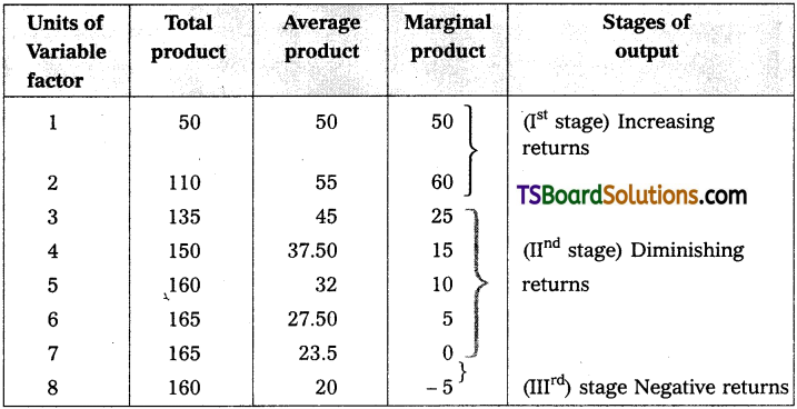
In the above table total product refers to the total output produced per unit of time by all the labourers employed.

Average product refers to the product per unit of labour marginal product refers to additional product obtained by employing an additional labour.

In the above table there are three stages of production.

1^st stage i.e., increasing returns at 2 units total output increases average product increases and marginal product reaches maximum.

2^nd stage i.e., diminishing returns from 3^rd unit onwards TP increases at diminishing rate and reaches maximum, MP becomes zero and AP continuously decreases.

3^rd stage i.e., negative returns from 8^th unit TP, decreases AP declines and MP becomes negative.

This can be explained in the following diagram.

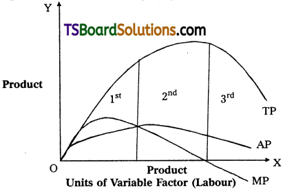
In the diagram, on ‘OX’ axis shown units labourer and ‘OY axis show TP, MP, and A.P. 1^st stage TP AP increases and MP is maximum. In the 2^nd stage TP is maximum, AP decreases and MP is zero. At 3^rd stage TP declines, AP also declines, MP becomes negative.

Question 2.
Explain the law of returns to scale. [Mar. ’17]
Answer:
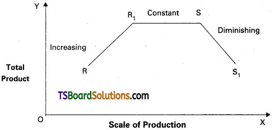
The law of returns to scale relate to long run production function. In the long run it is possible to alter the quantities of all the factors of production. If all factors of production are increased in given proportion the total output has to increase in the same proportion. Ex : The amounts of all the factors are doubled, the total output has to be doubled, increasing all factors in the same proportion is increasing the scale of operation. When all inputs are changed in a given proportion, then the output is changed in the same proportion. We have constant returns to scale and finally arises diminishing returns. Hence, as a result of change in the scale of production, total product increases at increasing rate, then at a constant rate and finally at a diminishing rate.

Assumptions :

1. All inputs are variable.
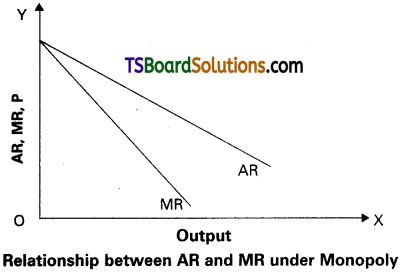
2. It assumes that state of technology remains the same. The returns to scale can be shown in the following table.

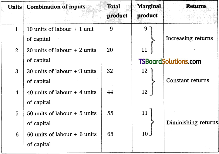
The above table reveals the three patterns of returns to scale. In the 1st place, when the scale is expanded upto 3 units, the returns are increasing. Later and upto 4^th units, it remains constant and finally from 5^th onwards the returns go on diminishing.

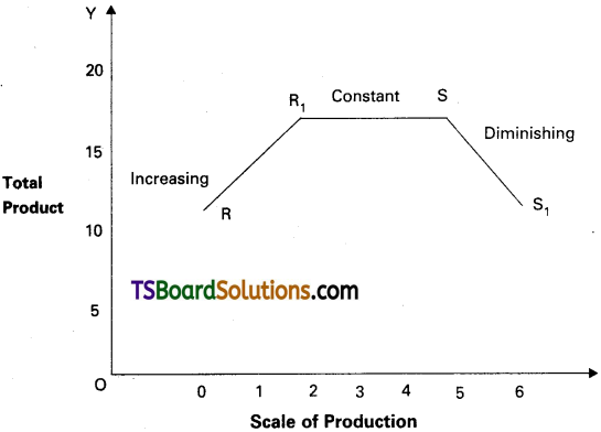
In the diagram, on ‘OX’ axis shown scale of production, on ‘OY’ axis shown total product. RR₁ represents increasing returns R₁S – Constant returns; SS₁ represents diminishing returns.

Question 3.
Describe the internal and external economies.
Answer:
Economies of large scale production can be grouped into two types.

1. Internal economies
2. External economies.

1. Internal Economies :
Internal economies are those which arise from the expansion of the plant, size or from its own growth. These are enjoyed by that firm only.

“Internal economies are those which are open to a single factory or a single firm independently of the action of other firms.” – Cairncross

i) Technological Economies :
The firm may be running many productive establishments. As the size of the productive establishments increase, some mechanical advantages may be obtained. Economies can be obtained from linking process to another process i.e., paper making and pulp making can be combined. It also uses superior techniques and increased specialization.

ii) Managerial Economies :
Managerial economies arises from specialisation of management and mechanisation of managerial functions. For a large size firm it becomes possible for the management to divide itself into specialised departments under specialised personnel. This increases efficiency of management at all levels. Large firms have the opportunity to use advanced techniques of communication, computers etc. All these things help in saving of time and improve the efficiency of the management.

iii) Marketing Economies :
The large firm can buy raw materials cheaply, because it buys in bulk. It can secure special concession rates from transport agencies. The product can be advertised better. It will be able to sell better.

iv) Financial Economies :
A large firm can arise funds more easily and cheaply than a small one. It can borrow from bankers upon better security.

v) Risk Bearing Economies :
A large firm incurs unrisk and it can also reduce risks. It can spread risks in different ways. It can undertake diversifications of output. It can buy raw materials from several firms.

vi) Labour Economies :
A big firm employs a large number of workers. Each worker is given the kind of job he is fit for.

2. External Economies :
An external economy is one which is available to all the firms in an industry. External economies are available as an industry grows in size.

i) Economies of Concentration :
When a number of firms producing an identical product are localised in one place, certain facilities become available to all. Ex : Cheap transport facility, availability of skilled labour etc.

ii) Economies of Information :
When the number of firms in an industry increases collective action and co-operative effort becomes possible. Research work can be carried on jointly. Scientific journal can be published. There is a possibility for exchange of ideas.

iii) Economies of Disintegration :
When the number of firms increases, the firm may agree to specialise. They may divide among themselves the type of products of stages of production. Ex : Cotton industry.

Question 4.
Explain short-run costs illustrations.
Answer:
Costs are divided into two categories i.e.,

1. Short run cost curves
2. Long run cost curves.

In short run by increasing only one factor i.e., (labour) and keeping other factor constant. The short run cost are again divided into two types.

1. General costs
2. Economic costs.

1. General Costs :
i) Money Costs :
Production is the outcome of the efforts of factors of production like land, labour, capital and organisation. So, rent to land, wage to labour, interest to capital and profits to entrepreneur has to be paid in the form of money is called money cost.

ii) Real Cost :
Adam Smith regarded pains and sacrifices of labour as real cost. So, it cannot be measured interms of money.

iii) Opportunity cost :
Factors of production are scarce and have alternative uses. The opportunity cost of a factor is the benefit that is foregone from the next best alternative use.

2. Economic Costs :
i) Fixed Costs :
The cost of production which remains constant even when the production may be increased or decreased is known as fixed cost. The amount spent by the cost of plant and equipment, permanent staff are treated as fixed costs.

ii) Variable Cost :
The cost of production which is changing according to changes in the production is said to be variable cost. In the long period all costs are variable costs. It includes prices of raw materials, payment of fuel, excise taxes etc. Marshall called it as “Prime cost”.

iii) Average Cost :
Average cost means cost per units of output. If we divided total cost by the number of units produced, we will get average cost.

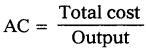
iv) Marginal Cost :
Marginal cost is the additional cost of production producing one more unit.
MC = \(\frac{\Delta \mathrm{TC}}{\Delta \mathrm{Q}}\)

v) Total cost :
Total cost is the sum of total fixed cost and total variable cost.
TC = FC + VC

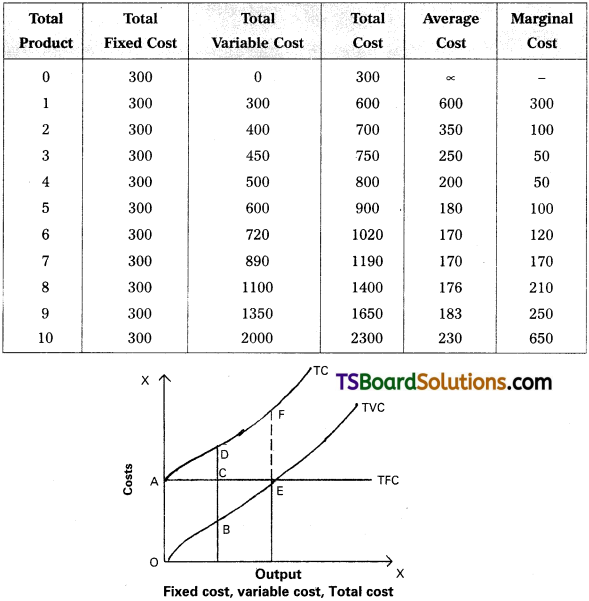
The short term cost in relation to output are explained with the help of a table.

In the above table shows that as output is increased in the 1^st column, fixed cost remains constant. Variable costs have changed as and when there are changes in output. To produce more output in the g TVC short period, more variable factors have to be employed. By adding FC & VC we get total cost at different levels of output. AC falls output increases, reaches its minimum and then rises MC also change in the total cost associated with a change in output. This can be shown in the diagram.

In the above diagram is on ‘OX’ axis taken by output and ‘OY axis is taken by costs. The shapes of different cost curves explain the relationship between output and different costs. TFC is horizontal to ‘X’ axis. It indicates that increase in output has no effect on fixed cost. TVC on the other side increases along with level of output. TC curve rises as output increases.

Question 5.
Write an essay on revenue analysis.
Answer:
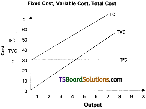
The amount of money that the producer receives in exchange for the goods (sale proceeds) is called producer’s receipts or revenue. In other words, the total sale proceeds of a firm are known as revenue. We can conceive three types of revenue. They are : total revenue, average revenue and marginal revenue.

a) Total Revenue (TR) :
Total amount of money or income received by the firm from the sale of a certain quantity of output is called total revenue. It is obtained by multiplying the price of a commodity by the number of units sold, i.e., TR = PQ.

Where, P = Price of the good and Q = the quantity of the good sold.

b) Average Revenue (AR) :
Average revenue is the revenue per unit of goods sold. It is computed by dividing the total revenue by the number of the units of a good sold. Thus, AR = TR / Q = PQ / Q = P. It is clear from the above formula that the average revenue at each level of output is equal to the price per unit.

c) Marginal Revenue (MR) :
It is the net addition to the total revenue by selling additional units of the goods i.e. the revenue which would be earned by selling an additional unit of the good. Marginal revenue can be expressed as : MR = ∆TR / ∆Q, where, ∆TR = change in total revenue and ∆Q = change in quantity. In other form, MR_n = TR_n – TR_n-1.

AR and MR Curves under Perfect Competition :
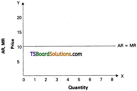
Under perfect competition, there exist large number of sellers and large number of buyers. The sellers under this competition offer homogenous products and, therefore, neither sellers nor buyers have any control on the price of the product. The seller can sell any amount of the good and buyers can buy any amount of the good at the ruling market price. In this case, total revenue (TR), average revenue (AR) and marginal revenue (MR) of a perfectly competitive firm are analyzed here under using table and diagram.

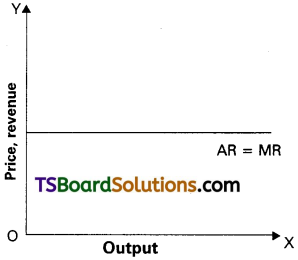
Since the price of the product remains constant under perfect competition, the output sold increases and therefore, revenue also increases. Due to homogeneity, the goods are sold at single price under perfect competition therefore, additional units are also sold at the same price. Hence, under this competition, the AR equals MR all through. Because of this, P = AR= MR. The nature of AR and MR curves is shown with the help of figure.

By the diagram, output is measured on OX axis and price / AR / MR on OY axis. OP price in the diagram indicates existence of single price. Since, P = AR = MR, the AR and MR curves will be parallel to OX axis as shown in figure.

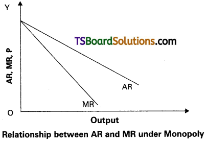
AR and MR Curves under Monopoly :
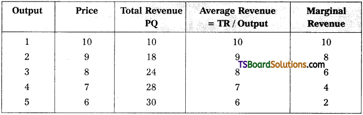
Under monopoly, there is a single seller. The commodity offered by a monoplist may be or may not be homogenous. Monopolist can control price and output of the commodity, but he can’t determine both simultaneously due to existence of left to right downward sloping demand curve in the market. He can sell more quantity at lower price and less quantity at higher price. The relationship between TR, AR and MR is shown in table.

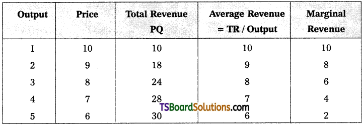
The table reveals that as price falls, sales may improve and total revenue also increases but average revenue (AR) and marginal revenue falls continuously. Here, MR declines at faster rate than that of AR. Thus, MR curve lies below the AR as shown in the figure.

In figure, AR and MR represent average revenue and marginal revenue curves re-spectively. The monopolist can sell higher quantity at lower price and therefore, always AR is greater than MR. Thus, AR curve lies above MR curve.

Short Answer Questions

Question 1.
Describe the main features of factors of production, namely land and labour.
Answer:
Land, labour, capital and entrepreneurial ability (organisation) are called as factors of production which make it possible to produce goods and services. The basic features of these factors of production are presented in the following paragraphs.

1) Land (N) :
The term land is used in a special sense in economics. It does not mean soil or earth’s surface alone but refers to all free gifts of nature which include besides land, in common practice, natural resources, fertility of soil, water, air, natural vegetation etc.

Characteristics of Land :
We may list the following characteristics of land as a factor of production.

• Land is a free gift of nature.
• The supply of land is perfectly inelastic from the point of view of the economy.
• Land cannot be shifted from one place to another place.
• Land is said to be a specific factor of production in the sense that it does not yield any result unless human efforts are employed.
• Land provides infinite variation of degree of fertility and situation so that no two pieces of land are exactly alike.

2) Labour (L) :
The term labour means mental or physical exertion directed to produce goods or services. In economics it is used in a wider sense. Any work, whether manual or mental, which is undertaken for a monetary consideration is called labour.

Characteristics of Labour :
Let us identify the characteristics of labour :

• Labour is inseparable from the labourer himself. It implies that whereas labour is sold, the producer of labour retains the capacity to work.
• Labour is highly ‘perishable’ in the sense that a day’s loss of labour cannot be stored and so he has no reserve price for his labour.
• Labour has a very weak bargaining power.
• Labour power differes from labourer to labourer. Therefore, labour may be classified as unskilled labour, semi skilled labour and skilled labour.
• The supply curve of a labourer is backward bending.

Question 2.
What are the merits and demerits of divisions of labour?
Answer:
It is an important feature of modern industrial organization. It refers to scheme of dividing the given activity among workers in such away that each worker is supposed to do one activity or only a limited and narrow segment of an activity. Thus, division of labour increases output per worker on account of higher efficiency and specialized skill.

Advantages :

1. Increase in productivity,
2. Inventions are facilitated,
3. Saving in time,
4. Diversity of employment,
5. Mechanization is possible,
6. Increase in dexterity and skills,
7. Large scale production is possible,
8. Right man in the right place.

Disadvantages :

1. Leads to monotony,
2. Retards human development,
3. Loss of skill,
4. Possibility of unemployment,
5. Hindrance to mobility of labour.

Question 3.
Explain the Diminishing Returns.
Answer:
Diminishing Returns :
After the stage of increasing returns, stage of diminishing returns will take place. This is known as the law of diminishing returns. Diminishing returns stage starts when the average product is maximum and continues upto the level of zero marginal product and maximum total product. Table shows this stage when the workers are employed from four to seven. From Q to Q₁ on OX axis shows the diminishing returns stage. In this stage, the total product increases at a diminishing rate and the average and marginal products decline. In this stage TP > AP > MP. Production is profitable only in the stage of diminishing returns.

Question 4.
Explain the concept of returns to scale.
Answer:
The law of returns to scale is concerned with the study of production function in the long run. The law of returns to scale studies the behaviour of output in response to change in scale. A change in scale means that all inputs or factors are varied in the same proportion, keeping the factor proportions constant. When a producer increases all the inputs in a given proportions, there are three possibilities, viz., total output may increase more than proportionately, just proportionately or less than proportionately. According to returns to scale concept, these possibilities are familiarly known as a) Increasing Returns To Scale (IRTS), b) Constant Returns To Scale (CRTS) and c) Decreasing Returns To Scale (DRTS).

Assumptions :

1. All inputs except entrepreneurship are variable.
2. State of technology remains the same.
3. There is perfect competition in the market.
4. Production is measured in physical quantities.

Explanation of the Law :
A description on returns to scale is presented in table. It can be seen from this table that the total product is 9 units in the beginning with 10L + IK. As the factors of production are doubled (20L + 2K), the total output increased to 19 units, which is more than proportional change and therefore, it represents increasing returns to scale (IRTS). Marginal product (MP) increased from 9 to 10 units uder this stage.

MP is remaining the same at 11 units when the scale is 30L + 3K and 40L + 4K therefore, it denotes constant returns to scale (CRTS). A decrease in MP is observed at 50L + 5K and 60L + 6K. This situation can be called as decreasing returns to scale (DRTS). These three kinds of returns to scale are also explained by using figure. In this figure, R to R₁ shows IRTS, R₁ to S shows CRTS and S to S₁ indicates DRTS.

Question 5.
Write a note on Capital.
Answer:
Capital as that part of wealth of an individual or a community which is used for further production of wealth. Capital (stock concept) yields periodical income (flow concept). Capital is nothing but ‘produced means of production’. The term capital is generally used for capital goods, E.g. plant and machinery, tools and accessories, stocks of raw materials, goods in process and fuel.

Types of Capital: Capital can be classified into :
1) Real Capital and Human Capital :
Real capital refers to physical goods, i.e., buildings, plant, machinery etc. As against this, human capital refers to human skill and ability.

2) Individual Capital and Social Capital :
Individual capital is the personal property, and the other, social capital is what belongs to the community as a whole in the form of roads, bridge etc.

3) Fixed Capital and Variable Capital :
Expenditure incurred on machinery and building in the production process is called as fixed capital. The amount spent on purchase of raw materials, daily wages to labour, electricity charges etc., are known as variable capital.

4) Tangible Capital and Intangible Capital :
Tangible capital may be perceived by senses where as intangible capital is in the form of certain rights and benefits. Eg. goodwill, patent rights, etc.

Importance of Capital :
Let us point out the importance of capital in brief.

1. Capital plays a very vital role in the modem productive system. Production without capital is almost impossible.
2. The productivity of work force depends upon the amount of capital available per worker. The greater the capital per worker, the greater the efficiency and productivity of the worker.
3. Capital occupies a central position in the process of economic development.
4. It promotes the technological progress.
5. It helps in the creation of employment opportunities.

Question 6.
What are the internal economies of scale?
Answer:
Economies of large scale production can be grouped under two headings. They are Internal economies and external economies. Let us discuss them.

Internal Economies :
The word ‘internal’ is used here to denote the limitations of these economies to the firm itself. According to Caimcross, “Internal economies are those which are open to a single factory or a single firm independently of the action of other firms”. Internal economies results in from an increase in the scale of output of a firm and cannot be achieved unless output increases. In other words, internal economies are those economies in production which accrue to the firm itself when it expands its output or enlarges its scale of production. In short, they arise simply due to the increase in the scale of production.

Firms experience the following types of internal economies :
a) Technical Economies :
Technical factors affect the returns to scale. Large firms will have more resources at their disposal. Therefore, these firms can install the most suitable machinery. As a result, larger firms experience lower costs of production. There are four different ways in which technical economies can arise. They are :

• large size machines,
• linking process, E.g. paper making and pulp making,
• superior techniques and
• increased specialization.

b) Managerial Economies :
With the increase in the scale of production, a firm can benefit by specializing its managerial department. Each department is under the charge of an expert. A small firm cannot afford this specialization. Experts are able to reduce the costs of production under their supervision.

c) Marketing Economies :
As the scale of a firm increases, internal economies accrue to the firm due to large scale purchases and sales. Since the firm purchases on a large scale, it gets all the inputs at a cheaper rate compared to the smaller firms. Similarly, wholesalers charge less for the sale of products to a large firm.

d) Financial Economies :
A large firm will be able to reduce its costs of borrowing from the market. A bigger firm is better known to the financial institutions and the stock market. Therefore, a big firm has better access to credit and can borrow on more favourable terms.

e) Economies of Welfare :
A big firm employes a large number of workers. Each worker is given the kind of job he is fit for. Therefore, workers get skilled in their operations which save production time and encourage new ideas.

f) Risk-Bearing Economies :
Large firms will be in a position to bear risks or avoid risks. They do so by diversifying output and markets. Therefore, loss in one good or in one market can be covered by profits in other goods or markets.

g) Economies of Research and Development :
Large firms possess more resources than small firms and hence, these firms invest huge amount of money on research and development (R & D). Introduction of innovative methods in production activity due to R & D reduces cost of production and results in internal economies.

Question 7.
What is supply? Explain the determinants supply.
Answer:
The law of supply explains the functional relationship between price of a commodity and its quantity supplied. The law of supply can be stated as follows, “Other things remaining the same, as the price of a commodity rises its supply is extended and as the price falls its supply is contracted”.

The law of supply can be explained with the help of supply schedule and supply curve.

Supply Schedule :
Supply schedule explains various amounts of good that the seller offers for sale at different prices. It represents the functional relationship between price and quantities supplied. There is direct relationship between price and supply. This can be shown in the following schedule.

Price (in ₹)	Quantity supplied
5.00	1000
4.00	800
3.00	600
2.00	400
1.00	200

The above schedule high price, i.e, ₹ 5.00 per unit, 1000 units are supplied and at ₹ 1 per unit, 200 units are supplied. It means high price indicate high supply and low price indicates low supply. So, it shows the direct relationship between price and supply.

Supply curve :
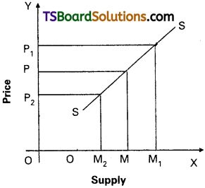
A supply curve can be drawn with the help of above supply schedule to explain the direct relationship between price and supply.

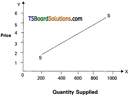
In the above diagram supply is shown on ‘OX’ axis and price is shown on OY axis. SS is supply curve. It slopes upwards from left to right; The slope of supply curve is always positive. Because there is direct relationship between the price and supply.

Determinants of Supply:
1. Price of the Commodity :
The supply of the commodity depends upon the price of that commodity. When price falls, supply falls and when price rises, supply also rises. Thus, price and supply are directly related.

2. Factor Prices :
The cost of production of a commodity depends upon the prices of various factors of production.

3. Prices of Related Goods :
The supply of the commodity depends upon the prices of related goods. If the price of a substitute good goes up, the producer will be induced to divert their resources.

4. State of Technology :
Technological improvements determine supply of a commodity. Progress in technology leads to reduction in the cost of production which will increase supply.

5. Government Policy :
Imposition of heavy taxes as a commodity discourages its production. Hence, production decreases.

Question 8.
Discuss about the changes in supply.
Answer:
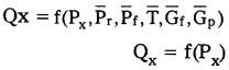
The supply function explains the relationship between the determinants of supply of a commodity and the supply of that commodity. Supply of a commodity depends upon its price, the prices of related goods, the prices of factors of production, the state of technology, the goals of firm and polity of the government. These can be written in the form a supply function as :
Q_x = f(P_x, P_r, P_f T, G_f, G_p)

Where, Q_x = quantity of good X supplied, P_x = price of good X, P_r = prices of related goods (substitutes, complementaries), P_f = prices of factors of production, T = technical knowhow, G_f = goal of the firm / seller, G_p = government policy, f = functional relationship.

In the above equation, supply of commodity is a dependent variable on many aspects. Change even in one variable of the determinants of supply brings a change in the supply. In determining the supply of a good, price of this good is more important among all the determinants. Hence, if we assume all other aspects will not change, then the supply function will be as :

Determinants of Supply :
Supply function explains the relationship between supply

i) Price of a Good :
In determining the supply of a good, price of this good is more important and this price determines the profit of the firm. Other things being constant, the supply of commodity increases with an increase in its price and vice versa. Thus, there exist a positive relationship between price and supply.

ii) Prices of its Related Goods :
Goods comprise substitutes and complementaries. Any change in the prices of these goods exerts influence on production of the good in consideration. For instance, if the price of a substitute good goes up, the producers may try to produce that substitute good or demand for the substitute good which has higher price may decrease and therefore, producer may increase supply of the good which he was producing initially. Similarly, producer may decide the supply of his product on the basis of the prices of complementaries and demand for them.

iii) Prices of Factors of Production :
Increase in the prices of factors of production would lead to an increase in the cost of production. As a result, supply of the commodity may decline. The reverse will happen in the case of a fall in the prices of factors of production.

iv) State of Technology :
New and improved methods of production, inventions and innovations help to save factors, costs and time and thus, technology contributes to increase the supply of goods.

v) Goals of producer and other determinants :
Goals of producer, means of transport and communication and natural factor etc., will equally influence the supply of a commodity.

vi) Government policy :
Imposition of heavy taxes on a commodity discourages the production of goods and as a result supply diminishes in goods are given, supply of goods will increase.

Question 9.
Discuss the types of costs.
Answer:
Cost analysis refers to the study of behaviour of production costs in relation to one or more production criteria, namely size of output, scale of operations, prices of factors of production and other relevant economic variable. In other words, cost analysis is concerned with financial aspects of production relations as against physical aspects considered in production analysis. A useful cost analysis needs a clear understanding of the various cost concepts which are dealt here under.

Types of Costs :
Broadly, types of costs can be classified into three types, namely, money costs, real costs and opportunity costs.

1) Money Costs :
The money spent by a firm in the process of production of its output is money cost. These costs would be in the form of wages and salaries paid to labour, expenditure on machinery, payment for materials, power, light, fuel and transportation. These costs are further divided into explicit costs and implicit costs. The amount paid to all factors of production hired from outside by the producer is called as explicit cost. And the amount of own resources and services applied by the producer in the production process is called as implicit cost.

2) Real Costs :
According to Alfred Marshall, “the pains and sacrifices made by labourers and entrepreneurs / organizers in the process of production activity are real costs”. The amount of crop (produce) sacrificed by the landlord by giving his land to tenants, the amount of leisure sacrificed by the labourer in extending labour to produce goods, the amount of consumption sacrificed by the investor by saving his money for investment are some of the examples of real costs.

3) Opportunity Costs :
It is also called as alternative cost or economic cost. Opportunity cost is next best alternative of factors of production. The alternate uses capacity of factors of production signifies opportunity costs. If a factor possesses alternative uses, the factor can be used only in one activity by forgoing other possibilities. In other words, opportunity cost is nothing but next best alternative foregone by a factor. For example, if a farmer decides to grow wheat instead of rice, the opportunity cost of the wheat would be the rice, which he might have grown rather. Thus, opportunity cost is the cost of foregone alternative.

Short-Run Cost Curve analysis :
In shortrun, the costs faced by a firm can be classified into fixed and variable costs.

4) Fixed Costs :
The fixed costs of a firm are those costs that do not vary with the size of its output. It is due to this, the value of fixed cost is always positive even if production activity does not take place or it is zero. The best way of defining fixed costs is to say that they are the costs which a firm has to bear even when it is temporarily shut down. Alfred Marshall called these costs as ‘Supplementary costs’ or ‘Overhead costs’. E.g.: costs of plant and equipment, rent on buildings, salaries to permanent employees are part of fixed costs.

5) Variable Costs :
On the other hand, Variable costs are those costs which change with changes in the volume of output. Marshall called these costs as ‘prime costs’. Daily wages to employees, payments to raw materials, fuel and power, excise taxes, interest on short-term loans etc., are examples for variable costs.

Question 10.
Explain the relationship between total cost, total variable cost and total fixed cost.
Answer:
In short-run, the costs faced by a firm can be classified into fixed and variable costs.

1) Fixed Costs and Variable Costs :
The fixed costs of a firm are those costs that do not vary with the size of its output. It is due to this, the value of fixed costs is always positive even if production activity does not take place or it is zero. The best way of defining fixed costs is to say that they are the costs which a firm has to bear even when it is temporarily shut down. Alfred Marshall called these costs as ‘Supplementary costs’ or ‘Overhead costs’. E.g.: costs of plant and equipment, rent on buildings, salaries to permanent employees are part of fixed costs. On the other hand, variable costs are those costs which change with changes in the volume of output. Marshall called these costs as ‘Prime costs’. Daily wages to employees, payment to raw materials, fuel and power, excise taxes, interest on short-term loans etc., are examples for variable costs.

2) Nature of short run Cost Curves :
As mentioned earlier, short-run is a period of time within which the firm can vary its output by varying only variable factors of production. The fixed factors such as capital equipment, top management personnel etc., cannot be varied. Therefore, short-run cost structure of a firm reveals fixed costs and variable costs, Total Cost (TC), Total Fixed Costs (TFC), Total Variable Costs (TVQ, Total Average Costs (SAC) and Marginal Costs (SMC). But in the long-run, all costs are variables. The nature of short-run costs and the curvature of these costs are explained by using table and figure.

In table, short-run costs faced by a firm are analyzed. As mentioned earlier, total fixed cost is the cost of fixed factors which remains constant irrespective of level of output. It is at ₹ 300/- Total variable cost, on the other hand, implies expenses on variable factors of production. It is zero when output is nothing or zero and goes on increasing along with the level of output. Total cost is the sum of total fixed cost and total variable cost i.e., TC = TFC + TVC. Though TFC remains constant, TVC increase along with the level of output, TC also increases if TVC increases. A description of the relationship between these three curves is presented in figure.

Question 11.
Explain the relationship between Average Cost and Marginal Cost.
Answer:
Cost analysis refers to the study of behavior of production costs in relation to one or more production criteria, namely, size of output, scale of operations, prices of factors of production and other relevant economic variables. In other words, cost analysis is concerned with financial aspects of production relations as against physical aspects considered in production analysis. A useful cost analysis needs a clear understanding of the various cost concepts which are dealt hereunder.

Relationship Between Average Cost and Marginal Cost :
Average cost (AC) is the sum of Average Variable Cost (AVC) and Average Fixed Cost (AFC). It is total cost divided by the number of units produced. In short, cost per unit is known as Average Cost (AC). AC = TC / Q = TFC / Q + TVC / Q = AFC + AVC. Marginal Cost (MC) is the addition made to the total cost by the production of additional units of output. It is the change in total cost associated with a change in output. We can therefore, write MC = Change in Total Cost / Change in Output = ∆TC / ∆Q or MC_n = TCn – TC_n-1

As per the nature of costs, both AC and MC curves gradually decrease, reach to mini-mum and gradually increase thereafter along with increase in level of output. It is to be noted that both AC and MC curves will have ‘U’ shape implying three phases i.e., decreasing, minimum (constant) and increasing. This is shown with the help of the following diagram.

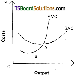
By the figure, output is measured on OX axis and costs on OY axis. It can be seen from this graph that in the beginning as output increases, both AC and MC decrease but the rate of decrease in MC is more than the decrease in AC. At point A, AC = MC and after this point both AC and MC increase but rate of increase in MC is greater than the rate of increase in AC.

Properties of AC and MC :

1. Both AC and MC curves are U shaped.
2. As output increases, both AC and MC decrease in the beginning.
3. MC curve cuts AC curve from its minimum points, at which point AC = MC.
4. Both AC and MC increase after certain level of output.

Question 12.
Explain diagramatically the nature of average revenue and marginal revenue under perfect competition and monopoly.
Answer:
The amount of money that the producer receives in exchange for the goods (sale proceeds) is called producer’s receipts or revenue. In other words, the total sale proceeds of a firm are known as revenue. We can conceive three types of revenue. They are : total revenue, average revenue and marginal revenue.

a) Total Revenue (TR) :
Total amount of money or income received by the firm from the sale of a certain quantity of output is called total revenue. It is obtained by multiplying the price of a commodity by the number of units sold, i.e., TR = PQ.
Where, P = Price of the good and Q = the quantity of the good sold.

b) Average Revenue (AR) :
Average revenue is the revenue per unit of goods sold. It is computed by dividing the total revenue by the number of the units of a good sold. Thus, AR = TR / Q = PQ / Q = P. It is clear from the above formula that the average revenue at each level of output is equal to the price per unit.

c) Marginal Revenue (MR) :
It is the net addition to the total revenue by selling additional units of the goods i.e., the revenue which would be earned by selling an additional unit of the good. Marginal revenue can be expressed as : MR = ∆TR / ∆Q, where, ∆TR = change in total revenue and ∆Q = change in quantity. In other form, MR_n = TR_n – TR_n-1.

AR and MR Curves under Perfect Competition:
Under perfect competition, there exist large number of sellers and large number of buyers. The sellers under this competition offer homogenous products and, therefore, neither sellers nor buyers have any control on the price of the product. The seller can sell any amount of the good and buyers can buy any amount of the good at the ruling market price. In this case, total revenue (TR), average revenue (AR) and marginal revenue (MR) of a perfectly competitive firm are analyzed here under using table and diagram.

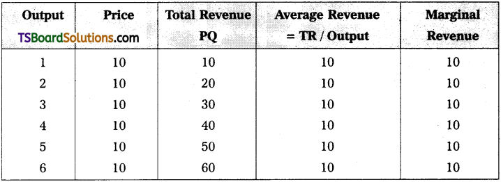
Since the price of the product remains constant under perfect competition, the output sold increases and therefore, revenue also increases. Due to homogeneity, the goods are sold at single price under perfect competition therefore, additional units are also sold at the same price. Hence, under this competition, the AR equals MR all through. Because of this, P = AR= MR. The nature of AR and MR curves is shown with the help of figure.

By the diagram, output is measured on OX axis and price / AR / MR on OY axis. OP price in the diagram indicates existence of single price. Since, P = AR = MR, the AR and MR curves will be parallel to OX axis as shown in figure.

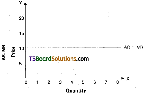
AR and MR Curves under Monopoly :
Under monopoly, there is a single seller. The commodity offered by a monoplist may be or may not be homogenous. Monopolist can control price and output of the commodity, but he can’t determine both simultaneously due to existence of left to right downward sloping demand curve in the market. He can sell more quantity at lower price and less quantity at higher price. The relationship between TR, AR and MR is shown in table.

The table reveals that as price falls, sales may improve and total revenue also increases but average revenue (AR) and marginal revenue falls continuously. Here, MR declines at faster rate than that of AR. Thus, MR curve lies below the AR as shown in the figure.

In figure, AR and MR represent average revenue and marginal revenue curves respectively. The monopolist can sell higher quantity at lower price and therefore, always AR is greater than MR. Thus, curve lies above MR curve.

Very Short Answer Questions

Question 1.
Explain the Characteristics of land.
Answer:
Land means not only earth’s surface alone but also refers to all free gits of nature which include soil, water, air, natural vegetation etc.

Characteristics of Land – The following are the characteristics of land as a factor of ‘ production
a) Free gift of nature.
b) Supply of land is perfectly inelastic.
c) Cannot be shifted from one place to another place.
d) Land provides infinite variation of degree of fertility.

Question 2.
What is Division of Labour?
Answer:
It is an important feature of modern industrial organisation. It refers to scheme of dividing the given activity among workers in such a way that each worker is supposed to do one activity or only a limited and narrow segment of an activity. Thus, division of labour increases output per worker on account of higher efficiency and specialised skill.

Question 3.
Define the Production Function.
Answer:
The production function is the relationship between the physical inputs and the physical outputs of a firm. Production of a firm, production function explains the functional relationship between inputs and outputs this can be as follows Gx = f (L, K, R, N, T).

Question 4.
Explain the concepts of Average Productand Marginal product
Answer:
It is the additional product by employing an additional labour.
MP = \(\frac{\Delta \mathrm{TP}}{\Delta \mathrm{L}}\)

It refers to the product per unit of labour it is obtained by dividing total product by the number of labourers employed.
Ap = \(\frac{TP}{L}\)

Question 5.
Explain the classification of Factors of production.
Answer:
Factors that help in the production process are called factors of production.
Ex : land, labour, capital and organization.

Question 6.
Explain the Technical economies.
Answer:
It is one of the internal economies.

The large firms will have more resources at their disposal. Hence, these firms can install the most suitable machinery. As a result larger firms experience lower cost of production. There are four different ways in which technical economies can arise.
a) Large size machines.
b) Linking processes.
c) Superior techniques.
d) Increased specialization.

Question 7.
What is the Importance of capital?
Answer:
Importance of Capital: The importance of capital in brief :

1. Capital plays a very vital role in the modem productive system. Production without capital is almost impossible.
2. The productivity of workforce depends upon the amount of capital available per worker. The greater the capital per worker, the greater the efficiency and productivity of the worker.
3. Capital occupies a central position in the process of economic development.
4. It promotes the technological progress.
5. It helps in the creation of employment opportunities.

Question 8.
Explain the External Economies.
Answer:
External economies are those economies which accure to each member firm as a result of the expension of the industry as a whole as the name tells us, these economies are common in nature which benefit all the firms working in an exponding industry external economies are as follows.
a) Economies of concentration.
b) Economies of information.
c) Economies of specialisation
d) Economies of welfare.

Question 9.
What is Capital Accumlation?
Answer:
Capital accumulation typically refers to an increase in assets from investment or profits. Individuals and companies can accumulate capital through investment. Investment assets usually earn profit they contributes to a capital base.

Question 10.
Define Supply function.
Answer:
Supply of a commodity depends upon a number of factors, the important among these can be presented in the form of a supply function. It explains the functional relationship between supply of a commodity and other determinants of supply of that commodity. This can be explained as follows.
S_x = f(P_x, P_y, P_f, T G_f, G_p)
S_x = Supply of commodity x
f = Functional relationship
P_x’ = Price of good x
P_y = Price of related good
P_f = Price of factors
T = Technical progress
G_f = Goal of the producer
G_p = Government policy.

Question 11.
Define Law of supply.
Answer:
The law of supply explains the functional relationship between price of a commodity and its quantity supplied. The law of supply can be stated as follows “Other things remaining the same, as the price of a commodity rises its supply is extended and as the price falls its supply is contracted”.

Question 12.
Explain the Supply schedule and supply Curve.
Answer:
Supply Schedule and Supply Curve :
The supply schedule is a table which explains various amounts of a good that the seller offered for sale at different prices. This table can be explained by the table as price increases from ₹ 30 to ₹ 60, the supply increases from 1,000 kgs to 4,000 kgs. It is to be noted that larger quantites are offered at a higher price than at a lower price.

Price (₹)	Quantity Supplied
30	1,000
40	2,000
50	3,000
60	4,000

Supply Curve :
Supply curve can be derived based on the supply schedule. By the diagram price is shown on Y – axis supply is shown on X – axis SS is the supply curve which slopes upwards from left to right. It implies that as price increases, supply also increases and vice versa. If price increases from p – p₁, supply also increases from M to M₁ and vice Versa.

Question 13.
What are Money costs? [Mar.’17]
Answer:
The money spent by a firm in the process of production of its output is money cost. These costs would be in the form of wages and salaries paid to labour, expenditure on machinery, payment for material, power, light, fuel and transportation. These costs are further divided into explicit costs and implicit costs.

Question 14.
What is an Opportunity cost?
Answer:
Opportunity cost :
It is also called alternative cost or economic cost. Opportunity cost is next best alternative use of factors of production. If a scarce factor possesses alternative uses, the factor can be used only in one activity by foregoing other possibilities. In other words, opportunity cost is nothing but next best alternative foregone by a factor. For example, if a farmer decides to grow wheat instead of rice, the opportunity cost of the wheat would be the rice, which he might have grown rather. Thus, opportunity cost is the cost of foregone alternative.

Question 15.
Describe the Total fixed cost curve.
Answer:
The fixed costs of a firm are those costs that do not vary with the size of its output. It is due to this the value of fixed costs is always positive even if production activity does not take place or it is zero. The best way of defining fixed costs is to say that they are the costs which a firm has to bear even when it is temporarily shut down. Alfred Marshall called these costs as supplementary costs or over head costs. For examples cost of plant and equipment, rent on building, salaries to permanent employees are part of fixed costs.

Question 16.
Explain the relationship between AC and MC.
Answer:
Average cost :
Average Cost (AC) is the sum of the Average Variable Cost (AVC) and Average Fixed Cost (AFC). It is total cost divided by the number of units produced. In short, cost per unit is known as average cost (AC).
AC = TC / Q = TFC / Q + TVC / Q = AFC + AVC.

Marginal Cost :
Marginal Cost (MC) is the addition made to the total cost by the production of additional units of output. It is the change in total cost associated with a change in output. We can therefore, write

MC = Change Total Cost / Change in Output or MC_n = TC_n – TC_n-1.

Question 17.
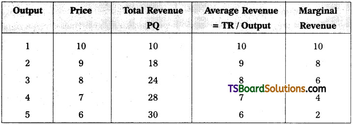
Explain the nature of AR and MR curves in perfect competition.
Answer:

Under perfect competition, there exist large number of sel1 rs and large number of buyers. In this market neither sellers nor buyers have any control on the price of the product. The seller can sell any amout of the good and buyers can buy any amount of the good at the ruling market price. Here the goods are sold at single price under perfect competition therefore, additional units are also sold at the same price. Hence, under perfect competition the AR = MR, because of this P = AR = MR. Since P = At = MR, the AR and MR curves will be parallel to OX axis as shown in the following diagram.

Question 18.
Explain the nature of AR and MR curves in Monopoly.
Answer:
Under monopoly, there is a single seller. The commodity offered by a monoplist may be or may not be homogenous. Monopolist can control price and output of the commodity, but he can’t determine both simultaneously due to existance of left to right downward sloping demand curve in the market. He can sell more quantity at lower pric e and less quantity at higher price. The relationship between TR, AR and MR is shown in table.

The table reveals that as price falls, sales may improve and total revenue also increases but average revenue (AR) and marginal revenue falls continuously. Here, MR declines at faster rate than that of AR. Thus, MR curve lies below the AR as shown in the figure.